A Survey of Mixup Method

• Mixup Method
  • Input Mixup
    • Results
  • Adaptive Mixup
  • Manifold Mixup
• The Application of Mixup Method
• Reference

FengHZ‘s Blog首发原创

In this article, we will give a brief review of mixup method which can dramatically improve the model performance with no extra computation. Mixup method now has played an important role in semi-supervised learning area, and we also provide a detailed implementation of all mixup methods in github.

Deep learning has achieved great success in supervised learning. The training process of deep learning can be formulated as the search of the function $f\in \mathcal{F}$ which maps the input space $\mathcal{X}$ to the label space $\mathcal{Y}$ that minimizes the expectation of the given loss $l(f(x),y)$

With the universal approximation theorem, the functional space $\mathcal{F}$ obtains any Borel measurable function from $\mathcal{X}$ to $\mathcal{Y}$. For the training dataset $\mathcal{D}={(x_i,y_i)_{i=1}^{n}}$, a natural thought is to use the empirical distribution function to estimate $dP(x,y)$ and induces the emperical risk minimization(ERM) target as follows

However the ERM risk $(2)$ monitors the behavior of f only at a finite set of n examples. When considering the universal approximation, one trival way to minimize $(3)$ is to force the network to simply overfit(memorize) the training data, which causes f to perform extremely poor in test dataset[1].

An simple way to improve $(2)$ is to use mixture gaussian distribution as the estimation of $dP(x,y$, which induces the following vicinal risk minimization(VRM) target

Mixup Method

Input Mixup

We can view $(3)$ as the operation that adds some noise $\epsilon \sim N(0,\sigma^2)$ to input, which is also called de-noising criterion. However, $(3)$ sill doesn’t give a natural form of $p_{y_i}(y)$ and the dirichlet function $\delta_{y_i}(y)$ is non-convex and rigorous. To solve this problem, [2] proposes a generic vicinal distribution called mixup:

In a nutshell, sampling from $\mu (x,y\vert \mathcal{D})$ can be simply written as

where $(x_i,y_i),(x_j,y_j)$ are two pairs randomly choosen from $\mathcal{D}$ and $\lambda$ is randomly sampled from $Beta(\alpha,\alpha)$. With sampled dataset $\mathcal{D}_{mixup}$, the related Mixup Risk Minimization (MRM) can be written as

\(R_{MRM}(f) = \frac{1}{m}\sum_{(x_i,y_i)\in \mathcal{D}_{mixup}} l(f(x_i),y_i)\)

Results

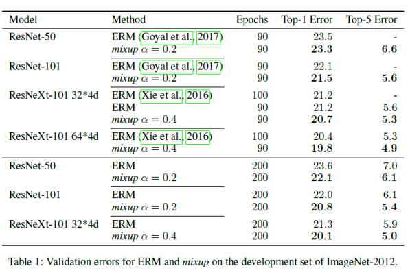
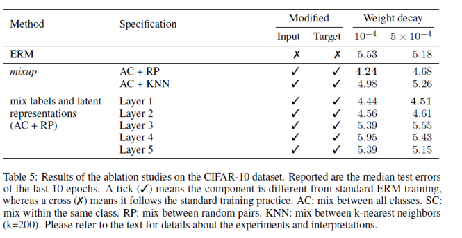
Utilizing the input mixup method can directly raise accuracy and improve the classification’s performance, just as the following tables show

Adaptive Mixup

The input mixup may meet the manifold intrusion problem when a mixed example collides with a real sample in the data manifold but the mixed label is very different from that of real sample. To figure out this problem, [3] proposes adaptive mixup strategy with policy region generator. Following is the schematic of Adaptive Mixup method

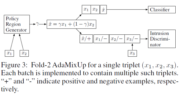
Firstly, we adversarially train a policy-region generator $PG$ to generate mixup parameter $\lambda$ and an intrusion discriminator $ID$ to distiguish the raw data $x$ and the mixed data $\tilde{x}$. Then we use $PG$ to generate $\lambda$ that can be classified as the mixed data by $ID$, and generate mixed data to train the classifier.

The author claims that with adaptive mixup, the network can achieve 3.52\% error in cifar10.

Manifold Mixup

The original mixup method only does interpolation in input space and the label space. But the linear interpolation in input space seems very anti-intuitive, and the arithmetic operations in feature space have shown more linear properties[4]. A natural way to improve input mixup is to do mixup in the middle layers of network, and the improvement is called manifold mixup.[5]

The mainfold mixup method has following 2 steps:

1. For each minibatch, select a random layer k which split the forward path of network into two parts: $N(x)=f_{k}g_{k}(x)$ and randomly sample $\lambda \sim Beta(\alpha,\alpha)$.

2. Minimize the manifold mixup risk minimization(MMRM) loss

   \[R_{MMRM}(f)= \sum_{(x_i,y_i),(x_j,y_j)\in \text{minibatch}} l(f_{k}(\lambda g_{k}(x_i)+(1-\lambda)g_{k}(x_j)),\lambda y_i + (1-\lambda)y_j) \tag{5}\]

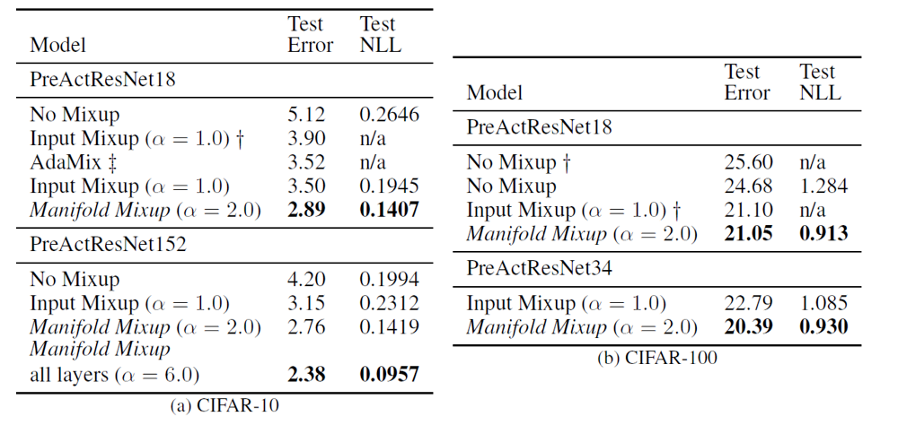
The selection strategy of parameter $\alpha$ for beta-distribution is extremely different from the input mixup method. In [2], the alpha is usually chose in range $[0.1,0.5]$, which will cause the probability mass of $\lambda$ to be concentrated on the endpoints of $[0,1]$. This strategy is very intuitive and is consistent with our visual cognition. But for manifold mixup, we usually choose $\alpha >1$, which makes $\lambda$ appear around 0.5 more likely.

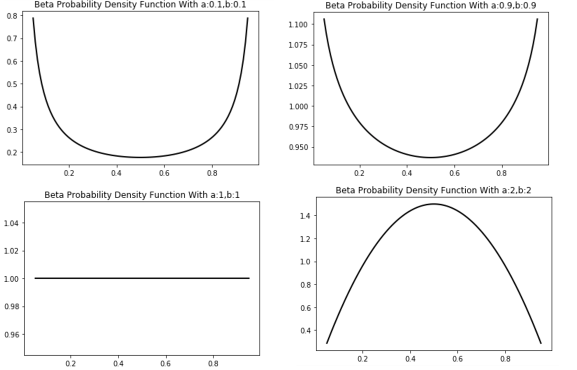
With appropriate $\alpha$, manifold mixup can make bigger improvements in classification performance than input mixup as the following states

The Application of Mixup Method

Besides directly improving model performance, mixup methods also have great potential in the following 3 areas

1. Robust to corrupted labels

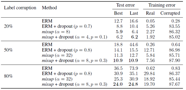
   [1] points out that the network just “memorizes” the label and the author claims that utilizing mixup method can relieve this problem. The two assumptions are

   • Increasing the strength of mixup interpolation $\alpha$ should generate virtual examples further from the training examples, making the memorization more difficult to achieve.

   • Learn interpolations between real examples is much easier than memorizing interpolations involving random labels.

And the results listed prove these assumptions

1. Robustness to Adversarial Examples

1. Semi-supervised Learning

   Mixup methods perform extremely well in semi-supervised learning tasks, which we have analyzed in this post.

Reference

1. Chiyuan Zhang, Samy Bengio, Moritz Hardt, Benjamin Recht, and Oriol Vinyals. Understanding deep learning requires rethinking generalization. arXiv preprint arXiv:1611.03530, 2016.

2. Zhang H, Cisse M, Dauphin Y N, et al. mixup: Beyond empirical risk minimization[J]. arXiv preprint arXiv:1710.09412, 2017.

3. Guo H, Mao Y, Zhang R. Mixup as locally linear out-of-manifold regularization[J]. arXiv preprint arXiv:1809.02499, 2018.

4. Tom White. Sampling generative networks. arXiv preprint arXiv:1609.04468, 2016.

5. Vikas Verma, Alex Lamb, Christopher Beckham, Amir Najafi, Ioannis Mitliagkas, David Lopez-Paz, and Yoshua Bengio. Manifold mixup: Better representations by interpolating hidden states. In International Conference on Machine Learning, pages 6438–6447, 2019.