Some Gradient Based Methods to Visualizing and Understanding CNN

• Introduction
• Transpose Convolution Method
• Gradient Based Method
  • Guided Back-propagation Method
  • Gradient Classification Activation Map Method
  • Global Average Pooling Method
  • Pixel-Wise Gradient-Guided Method
  • Result Analysis

FengHZ‘s Blog首发原创

Introduction

Large Convolutional Network models have recently demonstrated impressive classification performance and widely used in a range of medical image analysis tasks. However there is no clear understanding of why they perform so well, or what their judgement is based on.

Take an chest X-ray medical image as an example. To this image, an experienced radiologist will rely on the feature that the left thoracic cavity (on the right side of the image) has a sharp pleural boundary(the blue bounding box), while the right pleural boundary (on the left side of the image) has an obtuse angle and then diagnose pleural effusion. If we train an deep classification CNN model take it as input, the model will also make a diagnosis that it’s a patient with pleural effusion on the right part of the chest, while the process of prediction is a black box. The black box model may achieve high accuracy,whereas the lack of interpretability makes the model not directly usable in the clinic. Therefore, it’s important to make it clear what the diagnosis obtained from the model is based on.

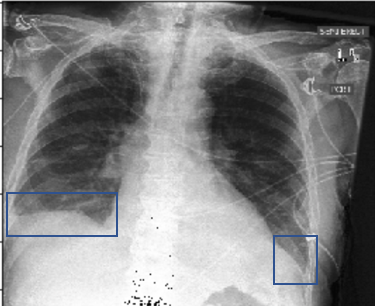
Here we discuss some CNN visualization methods based on the gradient of the target classification to open the black box. We will use the patient with pleural effusion as the basic example to compare the results of different methods. Our main references are

1. Visualizing and Understanding Convolutional Networks

2. Striving for simplicity: The all convolutional net

3. Learning deep features for discriminative localization

4. Grad-cam: Visual explanations from deep networks via gradient-based localization

Transpose Convolution Method

“Visualizing and Understanding Convolutional Networks” is the first paper proposing a visualization technique that maps middle feature into the original input space and gives insight into the function of intermediate feature layers. Though they don’t use the gradient method, their proposed thought “feature guide” that adds ReLU unit in the reconstruction process is very important. Their method is illustrated in the following figure

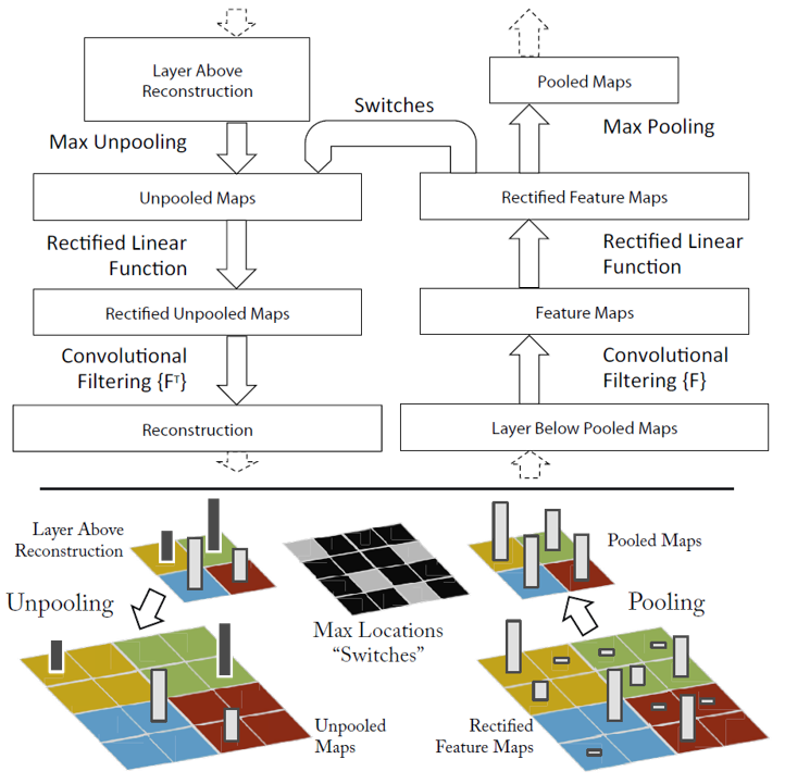
Suppose the model is composed of many convolution blocks and each block consists the following operations in sequence: convolution, relu, maxpool. For the i-th input feature $\mathbf{f^i}$, we calculate $\mathbf{f^{i+1}}$ in the following equation

Here we rewrite the convolution into the matrix multiplication form. Then the transpose convolution method map the feature $\mathbf{f^{i+1}}$ into the input space so that we can reconstruct the feature in the input space.

Notice the $\mathbf{F^T}$ operation is called “Transpose Convolution”, and ReLU operation plays a gradient-guiding role in the process of reconstruction which is used in all the next gradient based visualization methods. Suppose we want to visualization the k-th feature in l-th layer, then we just need to set $\mathbf{f^{l}}\in R^{CHW}$ to zero except the k-th feature, and use the transpose convolution method to map it into the input image space, and then we can see which part of the image does the feature encode exactly activate. Here are some examples

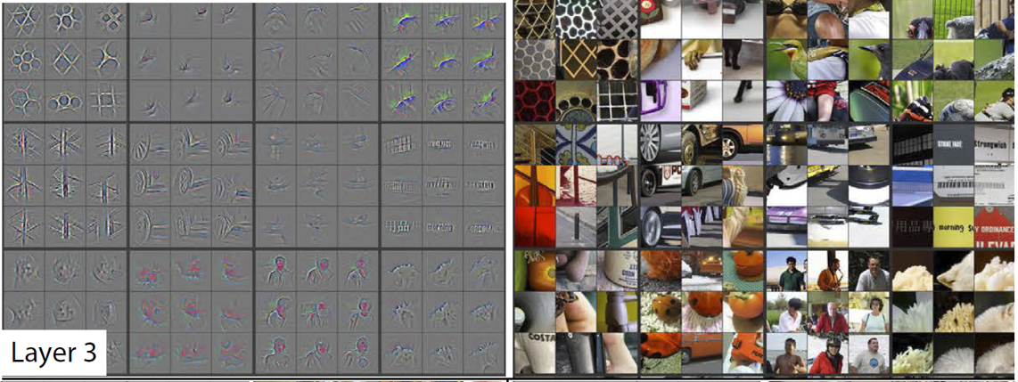
Take layer3 in alexnet for example, we visualize the most activated feature of the 3-rd layer in the input space. It seems that the feature captures the texture of some parts in the raw image as well as store the location information of the object.

Gradient Based Method

The transpose convolution method visualizes the information that middle features capture, but it doesn’t answer the interpretable question for a specific class c as we mentioned above. A nature thought is to use the quotient of the derivation of the classification score $y_c$ the derivation of the raw image $\mathbf{x}$

to see which changes in the image will lead to an increase in the classification confidence.

We can also look at $(1)$ from another distribution inference perspective. If we record the score vector as the inferenced posterior inference $q(\mathbf{y}\vert \mathbf{x})=multinomial(y_1,\ldots,y_c,\ldots)$ and the label vector as the true posterior distribution $p(\mathbf{y}\vert \mathbf{x}) = multinomial(0,\ldots,1,\ldots)$, then $(1)$ can be written as the negative gradient of $\mathcal{D}_{KL}[p\Vert q]$

The gradient is utilized to interprete reasons for the model to make a judgement in both fine-grained and coarse-grained modes.

Guided Back-propagation Method

Just as the name says, guided back-propagation method combines back-propagation and gradient-guiding operations, as shown in the following figure

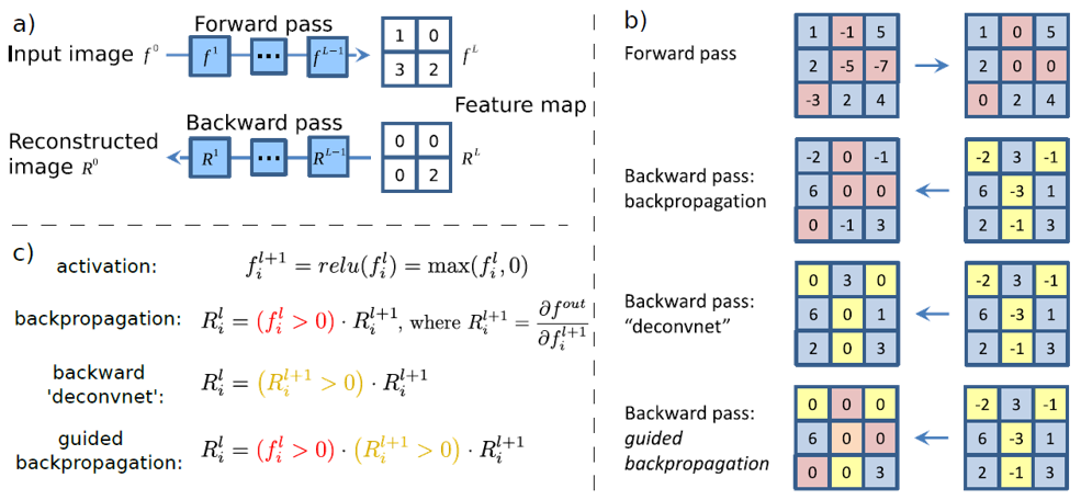
The gradient-guiding operation means to apply the ReLU operation to the gradient in back-propagation and the location where ReLU unit is applied is consistent with the position in the feed-forward way.

We take the patient with pleural effusion as example in order to see the result of this method and the role of the gradient-guiding operation.

In figure.c, this guided back-propagation method points out the same location as the doctor made the judgement. In figure.b, the result only gives the approximate location, which also indicates the reason why the ReLU operation on the gradient is called “guiding”.

The implementation of gradient-guiding operation is simple and we just need to slightly modify the original ReLU function as following

class _GuidedBackpropReLU(Function):

    def forward(self, input):
        positive_mask = (input > 0).type_as(input)
        output = torch.addcmul(torch.zeros(input.size()).type_as(input), input, positive_mask)
        self.save_for_backward(input, output)
        return output

    def backward(self, grad_output):
        input, output = self.saved_tensors
        grad_input = None

        positive_mask_1 = (input > 0).type_as(grad_output)
        positive_mask_2 = (grad_output > 0).type_as(grad_output)
        grad_input = torch.addcmul(torch.zeros(input.size()).type_as(input), torch.addcmul(torch.zeros(input.size()).type_as(input), grad_output, positive_mask_1), positive_mask_2)

        return grad_input

class GBReLU(nn.Module):
    def __init__(self,inplace=True):
        super(GBReLU,self).__init__()
        self.relu = _GuidedBackpropReLU()
    def forward(self,input):
        output = self.relu(input)
        return output

Gradient Classification Activation Map Method

In this part, we introduce a coarse-grained gradient-based activation map. The result of guided back-propagation method draws a fine-grained raw-image level visualization result, but it also has some problems. Take the last figure.c as an example, the result draws both the left and right thoracic cavity part, but only the right thoracic has pleural effusion. We can combine the fine-grained result and coarse-grained result to solve the problem and make the result more reasonable.

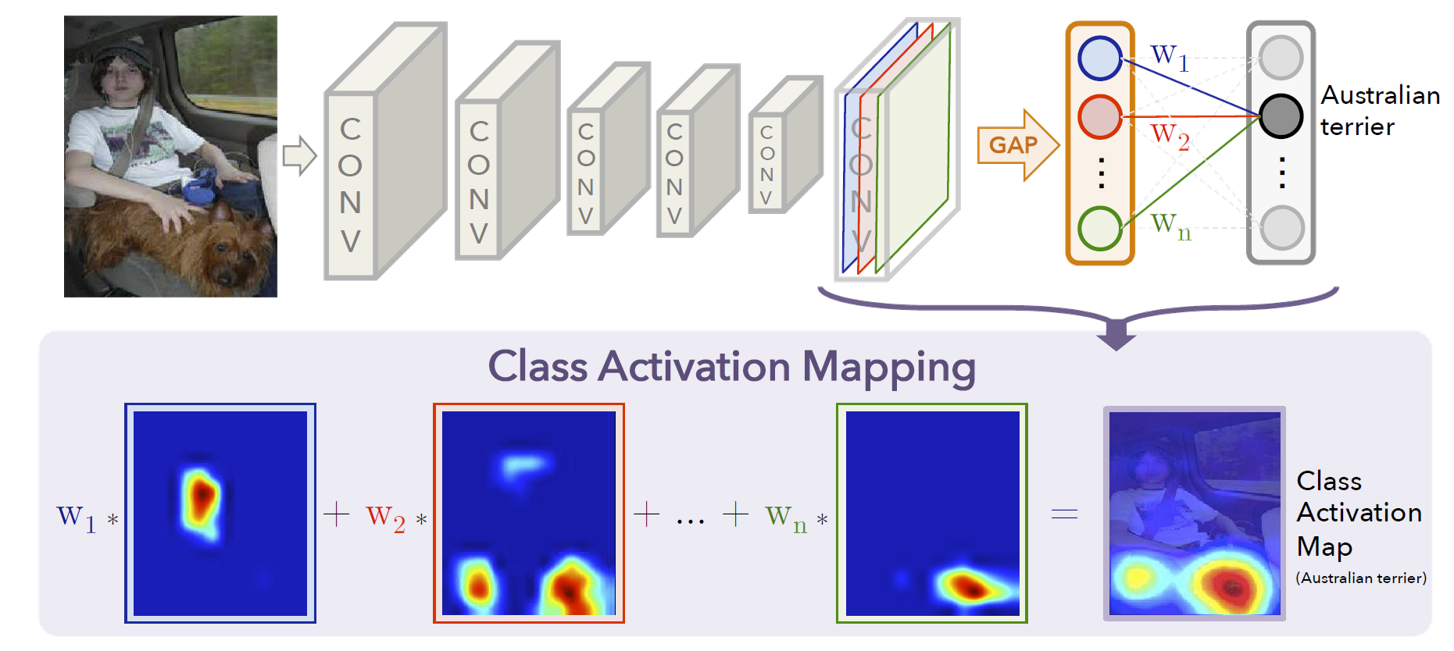
Notice that the convolution network is translation-invariant, and the last feature will preserve both the semantic level feature and the activated position information. So if we calculate gradient of the bottom feature space instead of the input space, we may get the coarse-grained level gradient activation combined with the position information.

For the last feature $\mathbf{F}\in R^{C\times H\times W}$, we calculate the gradient

and use $\mathbf{G}$ to get the weight for each channel in the last feature, just as the following figure illustrates

Global Average Pooling Method

We can use global average pooling method to calculate the weight

and get the activation map with equation

Pixel-Wise Gradient-Guided Method

We can also use the gradient $\mathbf{G}$ as the nature weight

or we can add gradient-guiding operation to improve the result

Result Analysis

Take the same example, we draw the coarse-grained visualization result combining with the fine-grained result in the following figure

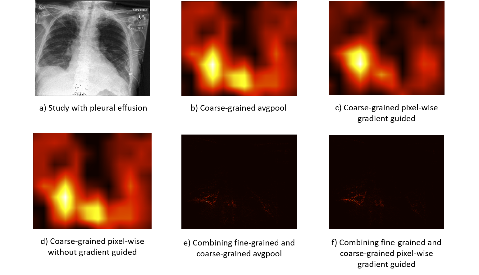
Comparing among the figure.b , figure.c and figure.d, we can find that the pixel-wise gradient-guided method have the most accurate location result, while the pixel-wise without gradient-guided method has the similar result to the global average pooling method, which indicates the importance of gradient-guiding operation.