Some Notes on the Decomposition of ELBO for VAE

• Introduction
• Commonly used forms of ELBO
  • Mutual information form
  • Disentangled form
  • Info-VAE
  • Decomposition for the assumptions
    • Use gan to measure the similarity
    • Use adversarial training to get the precise posterior distribution
• Applendix
  • Some notes on KL-Divergency
  • Proof for proposition 1.
  • Proof for proposition 2.
  • Proof for proposition 3.

FengHZ‘s Blog首发原创

Introduction

Variational autoencoders are usually combined of 2 parts: an encoder to predict the posterior of latent variable $z$ given input $x$ written as $q(z\vert x)$ and a decoder to predict the posterior of input $x$ given $z$ written as $p(x\vert z)$. Then we use the ELBO in statistical inference area to build loss function

where

To make $(2)$ have a closed form, we usually make some assumptions

However, the basic ELBO loss may have some difficulties in training and the assumptions for prior and posterior distributions are too strong in some ways. In this note, we introduce some different loss function forms by rewriting $(2)$ and impose some meta-prior by adding different weights to different components of loss.

Here we list some commonly used forms along with the proof. Our main references are

1. Recent Advances in Autoencoder-Based Representation Learning

2. Adversarial Variational Bayes: Unifying Variational Autoencoders and Generative Adversarial Networks

3. Autoencoding beyond pixels using a learned similarity metric

Commonly used forms of ELBO

At the beginning, we may declare some symbols and tricks as following

Mutual information form

We can rewrite $(2)$ in mutual information form as

proof :

Here we can get some insights from $(3)$. If we want to minimize $(3)$(as we want to minimize $(1)$), It appears that we need to minimize $I_{q_{\phi}}(x;z)$, which means the $x$ and $z$ will be independent and $z$ will not have enough information about $x$. So instead of minimize $(3)$ directly, we can give $I_{q_{\phi}}(x;z)$ a lower bound $C$ to make sure $z$ preserves enough information about $x$. In this opinion, we can rewrite the loss function $(2)$ as

Disentangled form

Based on $(3)$, we can add disentanglement as meta-prior. Assuming that the data is generated from independent factors of variation, for example object orientation and lighting conditions in images of objects, making disentanglement as a meta-prior encourages these factors to be captured by different independent variables in the representation. To encourage this representation, we can use the following rewriting form

proof :

A widely used notation for

is $TC(q_{\phi}(z))$. We can assign high weight to the part.1 loss to ensure the entanglement.

Info-VAE

Info-VAE rewrites the ELBO as the KL divergency of $q_{\phi}(z),p(z)$ and $q_{\phi}(x\vert z),p_{\theta}(x\vert z)$

proof :

Decomposition for the assumptions

To simplify the inference procedure, we proposes 2 assumptions separately for the prior and posterior distribution of latent variable $z$ and the posterior distribution of the input $x$ listed as following

However, it was observed that the reconstruction results often only vaguely resemble the input and the reconstruction result trained with mean square error only preserve the object considered salient and duplicate or average the small objects. To solve this problem, a set of adversarial methods have been proposed. Here we focus on 2 main methods target at $(4)$ and $(5)$ separately.

Use gan to measure the similarity

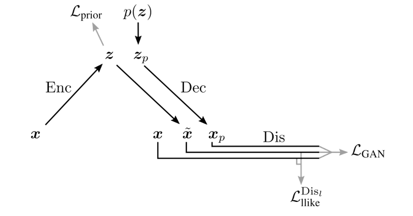
$(4)$ leads to the pixel-wise MSE Loss in the latent space, which is not very suitable for image data, as they do not model the properties of human visual perception. To deal with this problem, article combines GAN and VAE in reconstruction space to produce bette image samples. Following is the brief schematic.

We can rewrite $(2)$ as

The article adds a discriminator network to the original VAE and uses the output feature in the l-th layer of discriminator to calculate

as an alternative to $L^{pixel}_{llike}$.

The article also utilizes the discrimination loss for GAN

In the training proceduer, we use adversarial method to train Encoder, Decoder and Discriminator step by step. Following is the algorithm

• input $x$
• use Encoder to calculate $\mu_z,\Sigma_z$
• $L_{prior}=\mathcal{D}_{KL}(q(z\vert x)\Vert p(z))$
• use Decoder to calculate $x_{reconstruct}$
• sample $z\sim p(z)$, use Decoder to generate $x_{generate}$
• calculate the l-th output feature of Discriminator as $\text{Dis}_{l}(x)$ and then calculate \(L^{Dis_{l}}_{llike} = -\log p(\text{Dis}_{l}(x) \vert z)\)
• use Decoder to calculate $L_{GAN} = \log(\text{Dis}(x)) + \log(1-\text{Dis}(x_{reconstruct})) + \log(1-\text{Dis}(x_{generate}))$

• update the parameters step by step with SGD

  • \[\theta_{Encoder} \leftarrow -\nabla_{\theta_{Enc}}(L_{prior}+L^{Dis_{l}}_{llike})\]
  • \[\theta_{Decoder} \leftarrow -\nabla_{\theta_{Decoder} } (\gamma * L^{Dis_{l}}_{llike} - L_{GAN})\]
  • \[\theta_{Discriminator} \leftarrow -\nabla_{\theta_{Discriminator}} L_{GAN}\]

The article also proposes an indicator to quantify the quality of the generation result. If we get the inference of latent variables for all images, we can get the attribute vector use the mean and minus method for one attribute with 0-1 label for each image. Then we can generate images with this specific attribute using the attribute vector. We can train a classifier independently to distinguish the attribute, and use the ratio that the classifier successfully identify the generated image to measure the generation quality.

Use adversarial training to get the precise posterior distribution

The assumptions $(4)$ of the prior and posterior distribution of latent variable $z$ lead to the closed form of the second part in $(2)$

The assumption that $q_{\phi}(z\vert x)$ is taken to be a Gaussian distribution with diagonal covariance matrix whose mean and variance vectors are parameterized by neural networks with $x$ as input is very restrictive, potentially limiting the quality of the resulting generative model. Indeed, it was observed that applying standard Variational Autoencoders to natural images often results in blurry images(it may also be a result of the pixel-wise MSE loss in input space).

A simple improvement is to use the adversarial density-ratio estimation. Given a convex function $f$ for which $f(1)=0$, then the f-divergence between $p_{x}$ and $p_{y}$ is defined as

For $p_{y}(x)$ is the prior and always has a closed form, we can use adversarial trick to estimate the density ratio $\frac{p_{x}(x)}{p_{y}(x)}$, which can be expressed as

Notice here we assume $p(c=1)=p(c=0)$, so all we need is to train a discriminator to classify whether x is from $p_x$. Then we use the predicted score $S_{\eta}(x)$ to estimate the f-divergence and train VAE to minimize the f-divergence.

Another methood proposed in Adversarial Variational Bayes: Unifying Variational Autoencoders and Generative Adversarial Networks uses advsersarial method to get the exact value for

We build an discriminator $T(x,z)$ which takes $(x,z)$ as input and tries to distinguish pairs $(x,z)$ that were sampled independently using the distribution $\hat{p}(x)p(z)$ from those that were sampled using the current inference model, i.e., using $\hat{p}(x)q_{\phi}(z\vert x)$. The loss function for discriminator is described as following

Here, $\sigma(t)=\frac{1}{1+e^{-t}}$, and we have the first proposition to demonstrate the contribution of $(7)$

• Proposition 1. For $p_{\theta}(x,\vert z)$ and $q_{\phi}(z\vert x)$ fixed, the optimal discriminator $T^{\star}$ according to the objective in $(7)$ is given by \(T^{\star}(x,z) = \log q_{\phi}(z\vert x) -\log p(z) \tag{8}\) See the applendix for the details of the proof

Together with $(2)$, Proposition 1. allows us to write the ELBO as

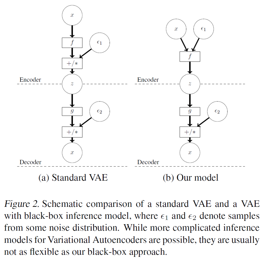
However, in $(9)$ we don’t give the analytical form of $q_{\phi}(z\vert x)$, so how to sample from $q_{\phi}(z\vert x)$ is a big question. The article modifies the basic VAE form and proposes an implicit sample method as the following schematic shows

Here we also use reparametrization trick but we inject noise on the top and let the learned function $f$ to do sample and inference together. Use this structure, we can directly sample $z$ using neural network with noise $\epsilon_1$. If we want to get another sample, then we just need to resample the noise $\epsilon_1$ and let the neural network predict $z \sim q_{\phi}(z\vert x)$.

To optimize $(9)$ we need to calculate the gradient with respect to $\theta$ and $\phi$. However, the parameter $\psi$ for $T^{\star}$ are optimized by $(7)$, which is related to $\phi$. But the gradient $\frac{\partial \psi}{\partial \phi}$ can’t be calculated directly, and we need the second proposition to handle this problem

• Proposition 2. We have \(E_{q_{\phi}(z\vert x)}[\nabla _{\phi}T^{\star}(x,z,\psi)=0]\) See the applendix for the details of the proof

Use the conclusion of Proposition 2, we can just fix the parameter $\psi$ in $T^{\star}$ and view $T^{\star}$ as an fixed optimization target. Then we can derive a target loss function for $\theta,\phi$ as following

Combined with $(7)$ , we can derive a two-player game with parameter $(\theta,\phi,\psi)$

And assume that $T$ can represent any function of two variables and $q_{\phi}(z\vert x)$ can represent any probability density on the latent space(universal approximation theorem in deep learning), if the $(\theta^{\star},\phi^{\star},\psi^{\star})$ defines a Nash-equilibrium of this two-player game, then we have the third proportion which decludes a beautiful, very strong and perfect result and gives us some useful and siginificant insights in the power of the adversarial method

• Proposition 3. Assume that $T$ can represent any function of two variables and $q_{\phi}(z\vert x)$ can represent any probability density on the latent space. If the $(\theta^{\star},\phi^{\star},\psi^{\star})$ defines a Nash-equilibrium of this two-player game, then we have

  • $(\theta^{\star},\phi^{\star})$ is the global optimum of the ELBO in $(2)$
  • $q_{\phi^{\star}}$ is equal to the true posterior $p_{\theta^{\star}}(z\vert x)$ (Powerful!)
  • $T^{\star}$ is the pointwise mutual information between $x$ and $z$, i.e. \(T^{\star}(x,z) = \log \frac{p_{\theta^{\star}}(x,z)}{p(x)p(z)}\)

  See the applendix for the details of the proof

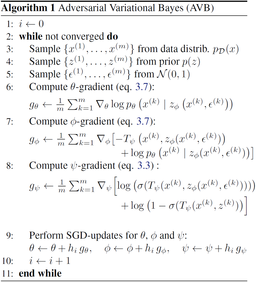
Based on the proposition 3, the article raises an algorithm for the adversarial strategy$(eq. 3.7 = (10),eq. 3.3 = (11))$

However, the stable training strategy of the algorithm is very difficult, for $T$ aims to distingush the two distribution $q_{\phi}(z\vert x) and p_{z}$, which are usually very different and easy to differentiate and will make discriminator too strong. To improve the quality of the estimate, the article propose to introduce an auxiliary conditional probability distribution $r_{\alpha}(z\vert x)$ with known density to approximates $q_{\phi}(z\vert x)$. We usually assume that $r_{\alpha}(z\vert x)$ is a Gaussian distribution with diagnoal covariance matrix whose mean and variance matches that of $q_{\phi}(z\vert x)$.

Utilizing this auxiliary distribution, we can rewrite ELBO as

In practice, we use $T$ to distinguish pair $(x,z)$ that sampled using $\hat{p}(x)r_{\alpha}(z\vert x)$ from pair $(x,z)$ that sampled using $\hat{p}(x)q_{\phi}(z\vert x)$, and we rewrite the two-players game $(10),(11)$ into the following form:

Here $T^{\star}(x,z_{\phi}(x,\epsilon))$ is supposed to be \(T^{\star}(x,z_{\phi}(x,\epsilon)) = \log q_{\phi}(z\vert x) -\log r_{\alpha}(z\vert x)\)

To estimate the mean and variance of $r_{\alpha}(z\vert x)$, we can simply sample $\epsilon$ many times and calculate the mean and std as the estimation. Another method is to use the network to predict $\mu$ and $\sigma$ for $z$ and do normalization with

then we can view

Following are the algorithm with adaptive contrast method

• Algorithm 2 Adversarial Variational Bayes with Adaptive Contrast

1. $i \leftarrow 0$
2. while not converged do
3. sample ${x^{(1)},\ldots,x^{(m)}}$ from $\hat{p}(x)$
4. sample ${\epsilon^{(1)},\ldots,\epsilon^{(m)}}$ from $\mathcal{N}(0,1)$
5. sample ${\eta^{(1)},\ldots,\eta^{(m)}}$ from $\mathcal{N}(0,1)$

6. for k =1,…,m do

7. \[z_{\phi}^{(k)},\mu^{(k)},\sigma^{(k)} =encoder_{\phi}(x^{(k)},\epsilon^{(k)})\]
8. \[\bar{z}_{\phi}^{(k)} = \frac{z_{\phi}^{(k)}-\mu^{(k)}}{\sigma^{(k)}}\]
9. end for

10. compute $\theta$-gradient

    \[g_{\theta} = \frac{1}{m}\sum_{k=1}^{m}\nabla_{\theta}\log p_{\theta}(x^{(k)}\vert z_{\phi}^{(k)})\]

11. compute $\phi$-gradient

    \[g_{\phi} = \frac{1}{m}\sum_{k=1}^{m}\nabla_{\phi}[-T_{\psi}(x^{(k)},\bar{z}_{\theta}^{(k)})+\log p_{\theta}(x^{(k)}\vert z_{\phi}^{(k)})+\frac{1}{2}\Vert \bar{z}_{\phi}^{(k)} \Vert^2 +\log p(\bar{z}_{\phi}^{(k)})]\]

12. compute $\psi$-gradient

    \[g_{\psi} = \frac{1}{m}\sum_{k=1}^{m} \nabla_{\psi}[\log \sigma(T_{\psi}(x^{(k)},\bar{z}_{\phi}^{(k)}))+\log (1-\sigma(T_{\psi}(x^{(k)},\eta^{(k)})))]\]
13. perform SGD-updates for $\theta,\phi,\psi$ with $g_{\theta},g_{\phi},g_{\psi}$
14. i = i+1
15. end while

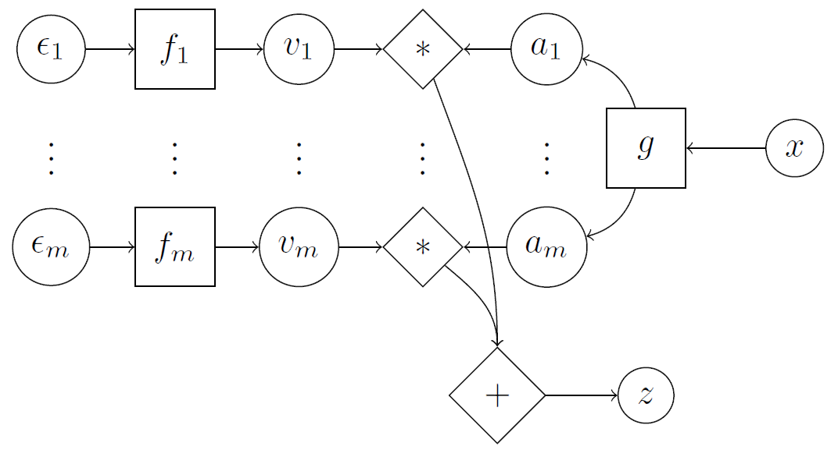
When it comes to how to combine $\epsilon$ with $x$, the article suggests the inner product

and we have

The details are illustrated in the following schematic

Applendix

Some notes on KL-Divergency

1. Suppose $p(z_1,\ldots,z_n)=\Pi p(z_j),q(z_1,\ldots,z_n)=\Pi q(z_j)$, then we have \(\mathcal{D}_{KL}(p\Vert q) =\sum_{j}\mathcal{D}_{KL}(p(z_j)\Vert q(z_j))\)

2. Suppose we only assume $q(z_1,\ldots,z_n)=\Pi q(z_j)$, then we have \(\mathcal{D}_{KL}(p\Vert q) =\mathcal{D}_{KL}[p(z)\Vert \Pi_{j}p(z_j)]+\sum_{j=1}^{n}\mathcal{D}_{KL}[q(z_j)\Vert p(z_j)]\)

Proof for proposition 1.

We can rewirte $(7)$ in an integral form

As the functions $\hat{p}(x),p(z),q_{\phi}(z\vert x)$ are given, we may rewrite $(A.1)$ as the limit form

A natural thought is that if we can get the maximum for each part

Then we can get the maximum of $(A.2)$. Utilizing the result that the function

achieves it’s maximum at $t=\frac{a}{a+b}$, so we can get that

and then use $\sigma(t)=\frac{1}{1+e^{-t}}$, we can get

Proof for proposition 2.

Use proposition 1, we have

Then

Here we use the conclusion $\nabla_{\phi}\int = \int\nabla_{\phi}$ without proof, but we can give a simple insight from the real analysis book written by Folland:

• Theorem 2.27 Suppose that $f:X\times [a,b] \rightarrow C(-\infty <a<b<\infty)$ and that $f(.,t):X\rightarrow C$ is integrable for each $t \in [a,b]$. Let $F(t)=\int_{X}f(x,t)d\mu(x)$. Suppose that $\frac{\partial f}{\partial t}$ exists and there is a $g\in L^{1}(\mu)(\text{note 1})$ s.t. that $\vert \frac{\partial f}{\partial t}(x,t) \vert \leq g(x)$ for all $x,t$. Then $F$ is differentiable and we have

  \[\frac{\partial F(t)}{\partial t} = \partial \int_{X}f(x,t)d\mu(x)/\partial t = \int_{X}\frac{\partial f(x,t)}{\partial t}d\mu(x)\]
  • note 1:definition We define $L^{1}(\mu)$ to be the collection of all complex measurable functions $f$ on $X$ for which
  \[\int _{X} \vert f\vert d\mu < \infty\]

Proof for proposition 3.

For given $(\theta^{\star},\phi^{\star})$e can easily get

which is illustrated in proposition 1. Inserting $(A.5)$ into $(10)$ shows that $(\phi^{\star},\theta^{\star})$ maximizes

which is equals to

Suppose the pair $(\phi^{\star},\theta^{\star})$ doesn’t maximize $(2)$, then there is another pair $(\phi^{‘},\theta^{‘})$ satisify that

and

which is contradict to the statement in $(A.6)$. So we have the pair $(\phi^{\star},\theta^{\star})$ maximizes $(2)$, which is correct if and only if